RMCTools has a auto tuner or gain optimizer that works very well most of the time. A question has been asked about how small changes affect the RMC’s ability to control position, velocity and acceleration. We use a simple linearized model for the hydraulic actuator’s open loop transfer function.
OLTF(s)=\frac { K\cdot { { { \omega }_{ n } } }^{ 2 } }{ s\cdot ({ s }^{ 2 }+2\cdot \zeta \cdot { \omega }_{ n }\cdot s+{ { { \omega }_{ n } } }^{ 2 }) }
K=10\quad (mm/s)/%\quad open\quad loop\quad gain
ζ = 0.3333333\quad damping\quad factor
{{ \omega }_{ n }} = 2*π*10\quad radians/second
s =\quad Laplace\quad operator
These parameters approximates moving a 2900 kg mass using a hydraulic cylinder 1000x63x40mm. The supply pressure is 200 bar and the valve is a 100 liter/min valve. This is a realistic load for testing.
So how much do varying loads and oil temperature changes affect motion?
One way to find out is to calculate the controller gains using the parameters above, then use these same parameters on a model where the parameters have changed by 10%. The RMC tuning wizard is much more accurate than +/- 10%.
So first I will make a move from 0 to 500mm at 500mm/s with an acceleration of 2500mm/s^2. The ramp time will be 0.2 seconds.
The open loop parameter are those listed above.
The controller gains are shown in the picture along with the mean squared error and the position error as a function of time.
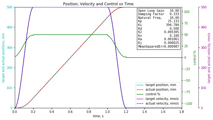
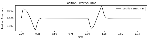
It is easy to see the response is too good. There is only about 0.002mm of error.
The next step is to execute the same code but reduce all the open loop parameters by 10% but still use the same gains. To be thorough there are 8 combinations to test where each gain is modified by +/- 10% . I have found that the worst combination occurs when all the gains are reduced by 10%.
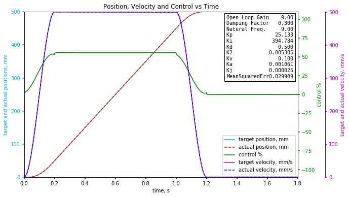
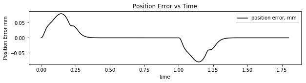
It is easy to see the following error has increased significantly from about 0.002mm to about 0.07mm but the absolute following error is still less than 0.1mm even while accelerating.
The reason why the following error is not bigger is due to the feedforwards making a pretty good estimate of the control output. The PID with second derivative gain allows higher gains than what can be achieved by using a PID or PI controller.
So what would cause the open loop parameters to drop by 10%?
From the VCCM equation it is easy to see the open loop gain will drop as a function of the square root of the supply pressure drop. This means that if the supply pressure drops to 81% of steady state the open loop gain will drop by about 10%. With proper accumulator sizing and charging the supply pressure should not drop more than 10% so the open loop gain will drop by only about 5%. If one wants to eliminate this error then use a pressure sensor to monitor the supply pressure. The output scale of the RMC controller can be modified on-the-fly to increase the controller gain to compensate for when the supply pressure drops.
The natural frequency can drop 10% if the mass increases by about 20%. Since the mass is in the denominator of the natural frequency equation and under a square root sign the mass can increase by about 20% resulting in the natural frequency dropping 10%.
System pressure variations have been the biggest issue with the nut staking machines we do the hydraulics and motion controls for. (RMC75).
Over 75% of the issues are with accumulators charge. These are very high cycle rate machines with force control as well. The customer is now installing sensors to check the charge pressure so they can do PM before the charge gets out of range instead of waiting for the parts to start checking bad.
The accumulator should not let the pressure drop by more than 10%.
If you look at the VCCM equation, you can see the open loop gain will vary by the square root of the pressure drop.
If the pressure drops to 81% of steady state pressure then the open loop gain will drop to 90% of the steady state open loop gain.
v_{ ss }=K_{ vpl }\sqrt { \frac { P_{ s }\cdot A_{ pe }-F_{ l } }{ A_{ pe }^{ 3 }\cdot (1+\frac { { \rho }_{ v }^{ 2 } }{ { \rho }_{ c }^{ 3 } } ) } }
If the supply pressure can be monitored then the output scale can be changed to compensate for pressure drops.
Multiply the output scale by
\sqrt { \frac { Ps0-Fl0 }{ Ps-Fl } }
Where
Ps0 and Fl0 are the steady state supply pressures and load.
Ps and Fl are the current pressures and load.
Eventually I will improve my Python simulator to be like my Mathcad simulator that simulates accumulators, pumps and valves.
deltamotion.com/peter/Mathcad/Ma … linder.pdf